How neurons actually look

We have all seen those pictures in the high school biology book - the cells in the nervous system, Neurons. Here I have shared some code snippets to visualize neurons (pulled from open source data) in their full glory.

Allen Institute for Brain Science shares a treasure trove of neuroscience related data with the community as well as the software support to access the data with Python. To get a feel of the different data modalitites please visit here. The data I am going to work with here is part of the Cell-types database. The neuron morphologies are digitally reconstructed from the images of mouse/human brain tissue slices and saved as .swc file. Please go here for a primer on the .swc format to understand how the measurements for the different sections of the neuron tree is saved.

Use AllenSDK to pull morphologies

We are going to use CellTypesCache() from the allensdk module to send a get request for cell id : 479225052. This particular cell comes from Layer 5 mouse visual cortex. For an overview of the physiology, morphology, metadata and all available computational models of this cell go here.

from allensdk.core.cell_types_cache import CellTypesCache
def get_morph_path(cell_id,save_filename=None):
    morph_path = save_filename or '%s.swc'%cell_id
    ctc = CellTypesCache()
    ctc.get_reconstruction(int(cell_id),file_name=morph_path)
    return morph_path 

cell_id = '479225052'
morph_path = get_morph_path(cell_id)

NeuroM

NeuroM is an open source tool from Blue Brain Project to analyze digitally reconstructed morphology. It comes with a visualization api which load files with extensions .swc/.h5/.asc.

import neurom.viewer
import matplotlib.pyplot as plt
fig,ax = neurom.viewer.draw(neurom.load_neuron(morph_path))
ax.grid(False)
ax.set_title('')
plt.show()

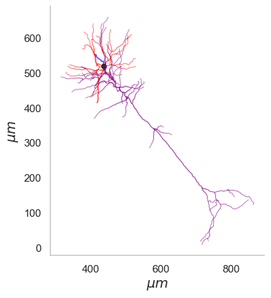
3D Visualization with transformation

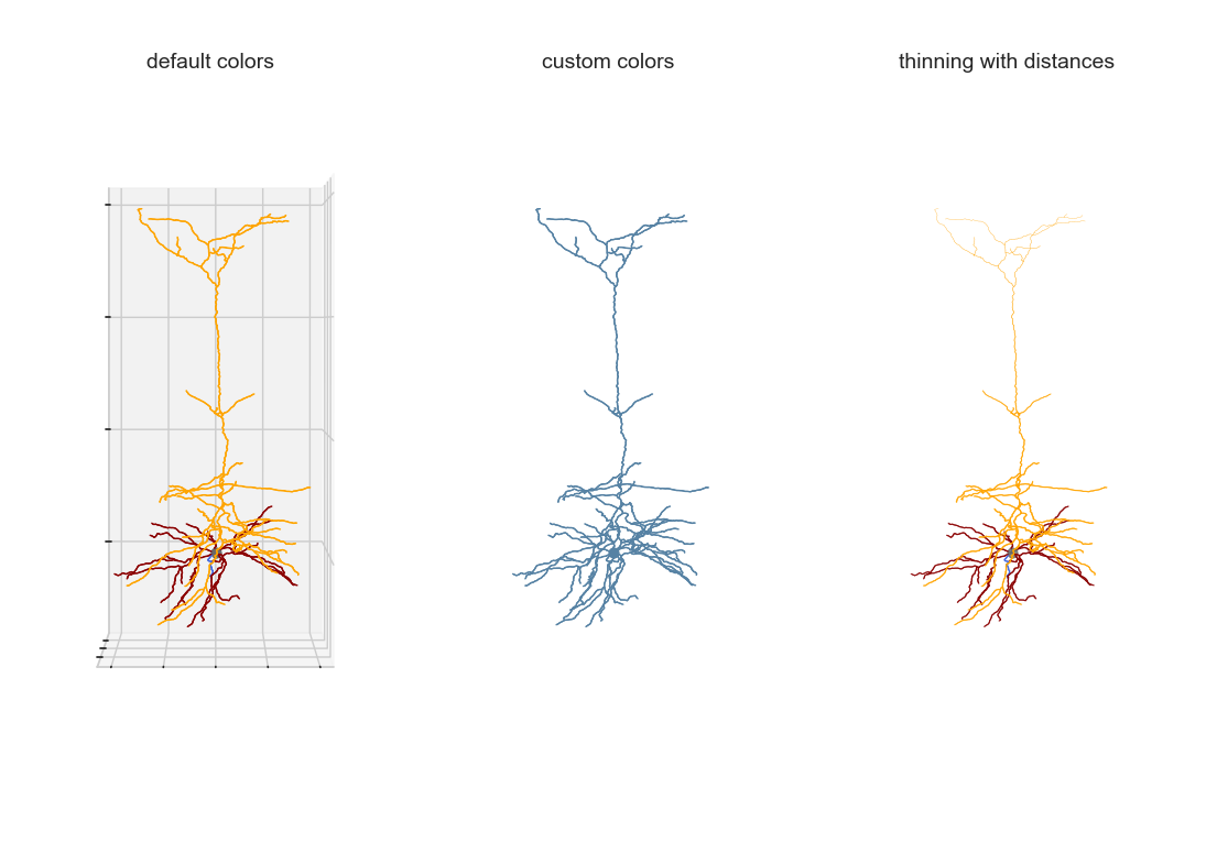
As part of a bigger project related to generating detailed biophysical models, I created some visualization tools for the morphologies . MorphHandler class offers the capability to rotate a neuron in 3D such that the apical trunk is upright. This involves computing the principal component of apical segments of the morphology and rotate the morphology along the axis normal to the plane composed of PC1 and positive z-axis = [0,0,1].

from ateamopt.morph_handler import MorphHandler
from mpl_toolkits.mplot3d import Axes3D
import seaborn as sns
morph_handler = MorphHandler(morph_path)
morph_data,morph_apical,morph_axon,morph_dist_arr = morph_handler.get_morph_coords()     
theta,axis_of_rot = morph_handler.calc_rotation_angle(morph_data,morph_apical)
fig = plt.figure()
ax = fig.add_subplot(projection='3d')
ax,_ = morph_handler.draw_morphology(theta,axis_of_rot,reject_axon=False,ax=ax)

Adding synapses and create animation

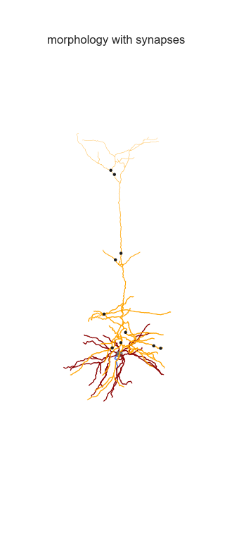
The MorphHandler class offers a basic synapse drawing method. Basically it plots specified number of synapses randomly on the desired sections.

ax,elev_angle = morph_handler.draw_morphology(theta,axis_of_rot,reject_axon=False,morph_dist_arr=morph_dist_arr,axis_off=True,alpha=.8)
n_syn_apical = 10
ax = morph_handler.add_synapses(morph_apical,n_syn_apical,theta,axis_of_rot,ax,color='k')
plt.show()

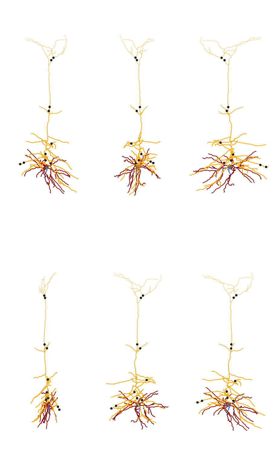
You can also animate the 3D morphology by rotating the camera angle around the z-axis. With the animation module we can pretty easily do that.

from ateamopt.animation import animation_module
angles = np.linspace(0,360,30)[:-1] # rotate the viewing position
files = animation_module.Animation.make_3Dviews(ax,angles,elevation=elev_angle,prefix='morph_anim/tmprot_')
movie_name = 'morph_movie_synapses.gif'
anim = animation_module.Animation(movie_name)
anim.make_gif(files,delay=20)

2D Visualization

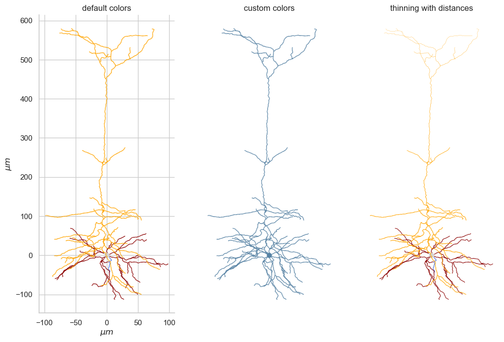
It’s straightforward to convert the 3d visualization to 2d within matplotlib. It’s as simple as projecting the morphology on xz or yz plane after rotation.

fig,ax=plt.subplots()
ax = morph_handler.draw_morphology_2D(theta,axis_of_rot,reject_axon=False,ax=ax)
plt.show()

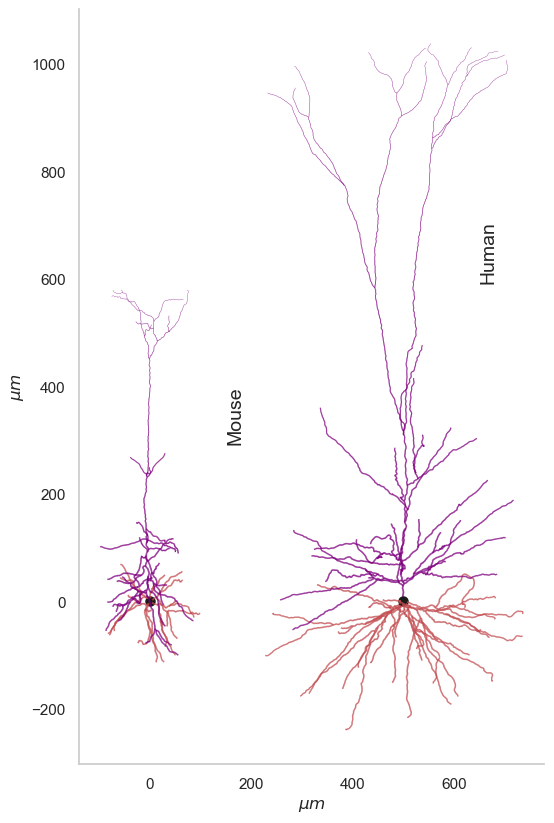
Comparison between Mouse and Human neuron

It’d be interesting how the mouse neuron matches up against a human one. I selected a pyramidal/excitatory cell (id : 571735073) from the cell-types database again. This neuron is part of excised epilieptic tissue within middle temporal gyrus from a human subject. As you might expect the human neurons are much bigger in size than mouse. For a scientifically rigorous cross species comparison check out this work from Allen Institute where the researchers look at transcriptomically homologous regions in mouse and human brain.

human_cell_id,mouse_cell_id = '571735073','479225052'
cell_ids = [mouse_cell_id,human_cell_id]
soma_displacement_x = 500
color_dict = {4: 'purple', 3: 'r', 2: 'b', 1 :'k' }
fig,ax = plt.subplots(figsize=(6,10))

for jj,cell_id in enumerate(cell_ids):
    morph_path = get_morph_path(cell_id)       
    morph_handler = MorphHandler(morph_path)
    morph_data,morph_apical,morph_axon,morph_dist_arr = morph_handler.get_morph_coords()
    soma_loc = np.array([jj*soma_displacement_x, 0])
    
    # Rotate morphology to appear upright                            
    theta,axis_of_rot = morph_handler.calc_rotation_angle(morph_data,morph_apical)
    ax = morph_handler.draw_morphology_2D(theta,axis_of_rot,soma_loc=soma_loc,color_dict=color_dict,morph_dist_arr=morph_dist_arr,ax=ax,lw=1.2,reject_axon=True)  

ax.set_xlabel('$\mu m$')
ax.set_ylabel('$\mu m$')
ax.text(150,300,'Mouse',rotation='vertical',fontsize=14)
ax.text(650,600,'Human',rotation='vertical',fontsize=14)
ax.grid(False)
sns.despine(ax=ax)
ax.grid(False)
plt.show()

Placing neurons along the mouse cortical depth

From the average depth of each layer we can place the neurons according to their normalized depth (0 corresponds to pia and 1 the white matter). The normalized depth is part of the metadata within Allen Cell-Types database. For a variety of cell-types (from a Cre-line sense) we iterate through the neurons and plot them in their respective layers.

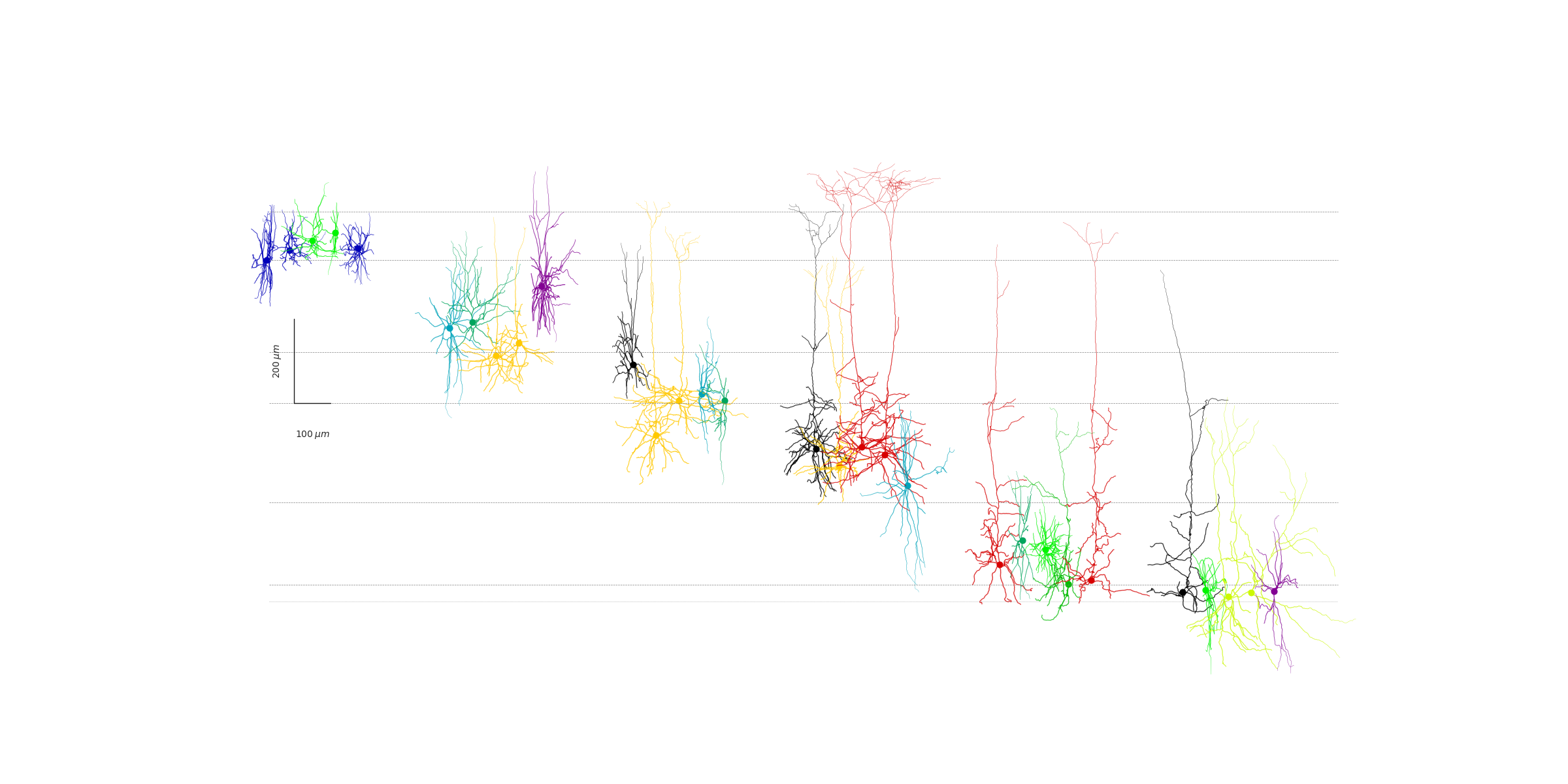
The entire notebook is shared here.